Microsoft Excel experience is so expected that it hardly warrants a line on a resume anymore. Then again how well do you actually know the way to use it?

Promoting and advertising and marketing is further data-driven than ever forward of. At any time you want to be tracking expansion charges, content material research, or advertising and marketing ROI. It’s conceivable you’ll know the way to plug in numbers and add up cells in a column in Excel, on the other hand that isn’t going to get you far when it comes to metrics reporting.

Do you want to understand what pivot tables are? Are you in a position for your first VLOOKUP? Aspiring Excel wizard, be informed on or leap to the segment that interests you most:

Table of Contents

• What’s Microsoft Excel?
• Microsoft Excel Spreadsheet Fundamentals
• Keyboard Shortcuts
• Pivot Tables
• IF Purposes
• VLOOKUP
• INDEX MATCH
• Knowledge Visualization

What’s Microsoft Excel?

Microsoft Excel is a popular spreadsheet instrument program for trade. It’s used for data get entry to and keep an eye on, charts and graphs, and challenge keep an eye on. You’ll be capable of construction, get ready, visualize, and calculate data with this device.

Learn to Download Microsoft Excel

It’s easy to acquire Microsoft Excel. First, check to ensure that your PC or Mac meets Microsoft’s gadget must haves. Next, take a look at in and arrange Microsoft 365.

After you take a look at in, practice the steps for your account and laptop gadget to acquire and unlock the program.

For example, say you’re working on a Mac desktop. You’ll be capable of click on on on Launchpad or look on your programs folder. Then, click on on on the Excel icon to open the application.

Microsoft Excel Spreadsheet Basics

Now and again, Excel seems too excellent to be true. Need to combine data in a few cells? Excel can do it. Need to copy formatting during an array of cells? Excel can do that, too.

Let’s get began this Excel data with the basics. After you have the ones functions down, you’ll be capable of tackle further professional Excel guidelines and complex courses.

Striking Rows or Columns

As you’re hired with data, it’s conceivable you’ll to search out yourself short of so that you can upload further rows and columns. Doing this one after the other might be super tedious. Happily, there’s an easier manner.

To be able to upload a few rows or columns in a spreadsheet, highlight the collection of pre-existing rows or columns that you want so that you can upload. Then, right-click and make a selection “Insert.”

In this example, I add 3 rows to the best of my spreadsheet.

Autofill

Autofill means that you can in short fill adjacent cells with quite a lot of types of data, along side values, series, and components.

There are many techniques to deploy this selection, on the other hand the fill take care of is likely one of the best.

First, choose the cells you want to be the availability. Next, to search out the fill take care of throughout the lower-right corner of the cell. Then each drag the fill take care of to cover the cells you want to fill or just double-click.

Filters

When you’re having a look at massive data gadgets, you most often don’t want to take a look at every row at the similar time. Now and again, you most efficient want to take a look at data that experience compatibility into certain requirements. That’s the position filters are to be had in.

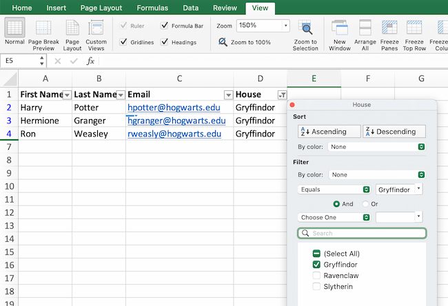
Filters will permit you to pare down data to only see certain rows at one time. In Excel, you’ll add a filter to each column on your data. From there, you’ll choose which cells you want to view.

To be able to upload a filter, click on at the Wisdom tab and make a selection “Clear out.” Next, click on at the arrow next to the column headers. This permits you to choose whether or not or now not you want to prepare your data in ascending or descending order, along with which rows you want to show.

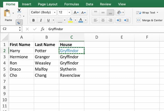
Let’s take a look at the Harry Potter example underneath. Say you most efficient wish to see the students in Gryffindor. By way of settling at the Gryffindor filter, the other rows disappear.

Skilled tip: Get began with a filtered view on your unique spreadsheet. Then, copy and paste the values to each different spreadsheet forward of you get began examining.

Kind

Now and again you’ll have a disorganized tick list of data. This is same old when you find yourself exporting lists, like promoting and advertising and marketing contacts or blog posts. Excel’s kind function imply you’ll alphabetize any tick list.

Click on on on the data throughout the column you want to type. Then click on on on the “Wisdom” tab on your toolbar and seek for the “Kind” selection on the left.

• If the “A” is on best of the “Z,” you’ll merely click on on on that button once. Choosing A-Z method the tick list will type in alphabetical order.
• If the “Z” is on best of the “A,” click on at the button two occasions. Z-A range method the tick list will type in reverse alphabetical order.

Remove Duplicates

Large datasets generally tend to have copy content material subject material. For example, you will have an inventory of quite a lot of company contacts, on the other hand you most efficient wish to see the collection of firms you will have. In situations like this, eliminating duplicates comes in handy.

To remove duplicates, highlight the row or column where you noticed copy data. Then, move to the Wisdom tab, and make a selection “Remove Duplicates” (underneath Apparatus). A pop-up will appear so that you can verify which data you want to stick. Make a choice “Remove Duplicates,” and you’re excellent to move.

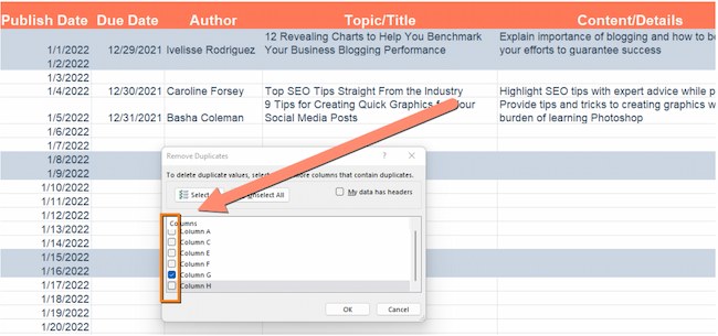
If you want to see an example, this post supplies step-by-step instructions for disposing of duplicates.

You’ll be capable of moreover use this selection to remove an entire row in line with a duplicate column worth. So, say you will have 3 rows of information and in addition you most efficient need to see one, you’ll make a selection all the dataset and then remove duplicates. The following tick list will have most efficient unique data without any duplicates.

Paste Specific

It’s steadily helpful to switch the items in a row of data appropriate right into a column (or vice versa). It is going to take numerous time to copy and paste each individual header.

Not to indicate, you want to merely fall into probably the most biggest, most unfortunate Excel traps — human error. Be told appropriate right here to take a look at one of the vital most now not extraordinary Microsoft Excel mistakes.

Instead of creating this kind of errors, let Excel do the provide the effects you need. Take a look at this case:

To use this function, highlight the column or row you want to transpose. Then, right-click and make a selection “Copy.”

Next, make a selection the cells where you want the main row or column to start out out. Right kind-click on the cell, and then make a selection “Paste Specific.”

When the module turns out, choose the technique to transpose.

Paste Specific is a smart useful function. Throughout the module, you’ll moreover choose between copying components, values, formats, or even column widths. This is specifically helpful when it comes to copying the results of your pivot table appropriate right into a chart.

Text to Columns

What if you want to minimize up out information this is in one cell into two different cells? For example, most likely you want to pull out any individual’s company determine via their email maintain. Or you want to separate any individual’s entire determine right into a number one and ultimate determine for your email promoting and advertising and marketing templates.

As a result of Microsoft Excel, each and every are conceivable. First, highlight the column where you want to split up. Next, move to the Wisdom tab and make a selection “Text to Columns.” A module will appear with more information. First, you need to make a choice each “Delimited” or “Mounted Width.”

• Delimited method you want to break up the column in line with characters harking back to commas, spaces, or tabs.
• Mounted Width method you want to make a choice the correct location in all the columns where you want the minimize as much as occur.

Make a choice “Delimited” to separate the total determine into first determine and ultimate determine.

Then, it’s time to select the delimiters. It is a tab, semicolon, comma, space, or something else. (For example, “something else” might be the “@” sign used in an email maintain.) Let’s choose the gap for this case. Excel will then show you a preview of what your new columns will seem to be.

When you’re pleased with the preview, press “Next.” This internet web page will allow you to make a choice Complicated Formats if you choose to. When you’re performed, click on on “Finish.”

Format Painter

Excel has numerous choices to make crunching numbers and examining your data speedy and easy. Then again should you ever spent some time formatting a spreadsheet, you realize it can get just a little tedious.

Don’t waste time repeating the identical formatting directions again and again. Use the construction painter to copy formatting from one area of the worksheet to each different.

To try this, choose the cell you’d like to copy. Then, make a selection the construction painter selection (paintbrush icon) from the best toolbar. When you free up the mouse, your cell should show the new construction.

Keyboard Shortcuts

Creating research in Excel is time-consuming enough. How can we spend a lot much less time navigating, formatting, and deciding on items in our spreadsheet? Glad you asked. There are a ton of Excel shortcuts to be had available in the market, along side a couple of of our favorites listed underneath.

Create a New Workbook

PC: Ctrl-N | Mac: Command-N

Make a choice Whole Row

PC: Shift-Space | Mac: Shift-Space

Make a choice Whole Column

PC: Ctrl-Space | Mac: Keep an eye on-Space

Make a choice Rest of Column

PC: Ctrl-Shift-Down/Up | Mac: Command-Shift-Down/Up

Make a choice Rest of Row

PC: Ctrl-Shift-Right kind/Left | Mac: Command-Shift-Right kind/Left

Add Hyperlink

PC: Ctrl-Adequate | Mac: Command-Adequate

Open Format Cells Window

PC: Ctrl-1 | Mac: Command-1

Autosum Determined on Cells

PC: Alt-= | Mac: Command-Shift-T

Excel Components

At this stage, you’re getting used to Excel’s interface and flying via speedy directions for your spreadsheets.

Now, let’s dig into the core use case for the instrument: Excel formulation. Excel imply you’ll do simple math like together with, subtracting, multiplying, or dividing any data.

• To be able to upload, use the + sign.
• To subtract, use the – sign.
• To multiply, use the * sign.
• To divide, use the / sign.
• To use exponents, use the ^ sign.

Bear in mind, all components in Excel could have initially an similar sign (=). Use parentheses to make sure certain calculations happen first. For example, consider how =10+10*10 isn’t like =(10+10)*10.

Besides manually typing in simple calculations, you’ll moreover discuss with Excel’s built-in components. One of the most most now not extraordinary include:

• Reasonable: =AVERAGE(cell range)
• Sum: =SUM(cell range)
• Depend: =COUNT(cell range)

Moreover phrase that series’ of explicit cells are separated by the use of a comma (,), while cell ranges are notated with a colon (:). For example, you want to make use of any of the ones components:

• =SUM(4,4)
• =SUM(A4,B4)
• =SUM(A4:B4)

Conditional Formatting

Conditional formatting means that you can change a cell’s color in line with the information throughout the cell. For example, say you want to flag a category on your spreadsheet.

To get started, highlight the crowd of cells you want to use conditional formatting on. Then, choose “Conditional Formatting” from the Space menu. Next, make a selection a commonplace sense selection from the dropdown. A window will pop up that turns on you to offer further information about your formatting rule. Make a choice “OK” when you find yourself performed, and in addition you should see your results routinely appear.

Follow: You’ll be capable of moreover create your personal commonplace sense if you want something previous the dropdown conceivable alternatives.

Greenback Signs

Have you ever ever ever seen a dollar take a look at in an Excel device? When this symbol is in a device, it isn’t representing an American dollar. Instead, it makes sure that the correct column and row stay the identical although you copy the identical device in adjacent rows.

You notice, a cell reference — when you discuss with cell A5 from cell C5, for instance — is relative by the use of default.

This means you’re actually when it comes to a cell this is 5 columns to the left (C minus A) and within the identical row (5). That is referred to as a relative system.

When you copy a relative device from one cell to each different, it’s going to adjust the values throughout the device in line with where it’s moved. Then again now and again, you want those values to stay the identical irrespective of whether or not or now not they’re moved spherical or no longer. You’ll be capable of do that by the use of making the device throughout the cell into what’s referred to as an absolute device.

To change the relative device (=A5+C5) into an absolute device, precede the row and column values with dollar signs, like this: (=$A$5+$C$5).

Combine Cells Using “&”

Databases generally tend to split out data to make it as actual as conceivable. For example, instead of having data that presentations a person’s entire determine, a database would most likely have the guidelines as a number one determine and then a last determine in separate columns.

In Excel, you’ll combine cells with different data into one cell by the use of using the “&” sign on your function. The example underneath uses the program: =A2&” “&B2.

Let’s move during the device together using an example. So, let’s combine first names and ultimate names into entire names in a single column.

To try this, put your cursor throughout the blank cell where you want the total determine to seem. Next, highlight one cell that comprises a number one determine, kind in an “&” sign, and then highlight a cell with the corresponding ultimate determine.

Then again you at the moment are now not finished. If all you kind in is =A2&B2, then there is probably not a space between the person’s first determine and ultimate determine. To be able to upload that very important space, use the function =A2&” “&B2. The quotation marks around the space tell Excel to position a space between the main and ultimate determine.

To make this true for a few rows, drag the corner of that first cell downward as confirmed throughout the example.

Pivot Tables

Pivot tables reorganize data in a spreadsheet. A pivot table may not change the guidelines that you simply’ve were given, on the other hand it would sum up values and read about information by hook or by crook this is easy to understand.

For example, let’s check out how many people are in each area at Hogwarts.

To create the Pivot Table, move to Insert > Pivot Table. Excel will routinely populate your pivot table, on the other hand you’ll at all times change the order of the guidelines. Then, you will have 4 alternatives to choose from.

Record Clear out

This allows you to most efficient take a look at certain rows on your dataset.

For example, to create a filter by the use of area, choose most efficient students in Gryffindor.

Column and Row Labels

The ones might be any headers or rows throughout the dataset.

Follow: Every Row and Column labels can include data from your columns. For example, you’ll drag First Determine to each the Row or Column label depending on how you want to look the guidelines.

Value

This segment allows you to convert data into a bunch. Instead of merely pulling in any numeric worth, you’ll sum, rely, average, max, min, rely numbers, or do a few other manipulations along side your data. By way of default, when you drag a field to Value, it at all times does a rely.

The example above counts the collection of students in each area. To recreate this pivot table, move to the pivot table and drag the Area column to each and every the row Labels and the values. This may increasingly sum up the collection of students associated with each area.

IF Functions

At its most basic degree, Excel’s IF function means that you can see if a state of affairs you set is correct or false for a given worth.

If the placement is correct, you get one end result. If the placement is faux, you get each different end result.

This commonplace device turns out to be useful for comparisons and finding errors. Then again should you’re new to Excel you want to need reasonably more information to get necessarily essentially the most out of this selection.

Let’s take a look at this function’s syntax:

• =IF(logical_test, value_if_true, [value_if_false])

• With values, this might be: =IF(A2>B2, “Over Price range”, “OK”)

In this example, you want to hunt out where you’re overspending. With this IF function, if your spending (what’s in A2) is larger than your finances (what’s in B2), that overspending could be easy to look. You then’ll then filter the guidelines so that you understand most efficient the street items where you’re going over finances.

The real power of the IF function comes when you string or “nest” a few IF statements together. This allows you to set a few must haves, get further explicit results, and get ready your data into further manageable chunks.

For example, ranges are one way to segment your data for upper analysis. For example, you’ll categorize data into values which could be less than 10, 11 to 50, or 51 to 100.

=IF(B3<11,”10 or a lot much less”,IF(B3<51,”11 to 50″,IF(B3<100,”51 to 100″)))

Let’s discuss a few further IF functions.

COUNTIF Function

The power of IF functions goes previous simple true and false statements. With the COUNTIF function, Excel can rely the collection of events a word or amount turns out in any range of cells.

For example, let’s think you want to rely the collection of events the word “Gryffindor” turns out in this data set.

Take a look at the syntax.

• The device: =COUNTIF(range, requirements)
• The device with variables from the example underneath: =COUNTIF(D:D,”Gryffindor”)

In this device, there are a selection of variables:

Range

The variability that you want the device to cover.

In this one-column example, “D:D” presentations that the main and ultimate columns are each and every D. If you want to take a look at columns C and D, use “C:D.”

Requirements

Regardless of amount or piece of text you want Excel to rely.

Best possible use quotation marks if you want the end result to be text instead of a bunch. In this example, “Gryffindor” is the only requirements.

To use this function, kind the COUNTIF device in any cell and press “Enter.” Using the example above, this movement will show how over and over the word “Gryffindor” turns out throughout the dataset.

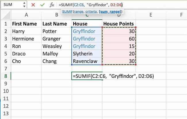
SUMIF Function

Ready to make the IF function just a little further complex? Let’s say you want to investigate the collection of leads your blog has generated from one writer, no longer all the group of workers.

With the SUMIFS function, you’ll add up cells that meet certain requirements. You’ll be capable of add as many quite a lot of requirements to the device as you like.

Proper right here’s your device:

• =SUMIFS(sum_range, criteria_range1, criteria1, [criteria_range2, criteria 2],and so on.)

That’s numerous requirements. Let’s take a look at each segment:

Sum_range

The number of cells you’re going so that you can upload up.

Criteria_range1

The variability that is being searched for your first worth.

Criteria1

That’s the explicit worth that determines which cells in Criteria_range1 so that you can upload together.

Follow: Bear in mind to use quotation marks should you’re looking for text.

Throughout the example underneath, the SUMIF device counts the total collection of area problems from Gryffindor.

IF AND/OR

The OR and AND functions round out your IF function conceivable alternatives. The ones functions check a few arguments. It returns each TRUE or FALSE depending on if at least probably the most arguments is correct (that’s the OR function), or if all of them are true (that’s the AND function).

Out of place in a sea of “and’s” and “or’s”? Don’t check out however. In observe, OR and AND functions received’t ever be used on their own. They need to be nested inside of each different IF function. Recall the syntax of a basic IF function:

• =IF(logical_test, value_if_true, [value_if_false])
• Now, let’s fit an OR function throughout the logical_test: =IF(OR(logical1, logical2), value_if_true, [value_if_false])

To place it it appears that evidently, this combined device allows you to return a price if each and every must haves are true, as opposed to just one. With AND/OR functions, your components may also be as simple or complex as you want them to be, as long as you understand the basics of the IF function.

VLOOKUP

Have you ever ever ever had two gadgets of data on two different spreadsheets that you want to combine appropriate right into a single spreadsheet?

For example, say you will have an inventory of names and email addresses in one spreadsheet and an inventory of email addresses and company names in a definite spreadsheet. Then again you want the names, email addresses, and company names of those other folks to seem in one spreadsheet.

VLOOKUP is a smart go-to device for this.

Faster than you employ the device, be sure that you will have at least one column that appears identically in each and every places.

Follow: Scour your data gadgets to make sure the column of data you’re using to combine spreadsheets is strictly the identical. This accommodates eliminating to any extent further spaces.

Throughout the example underneath, Sheet One and Sheet Two are each and every lists with different information about the identical other folks. The common thread between the two is their email addresses. Let’s combine each and every datasets so that all the area information from Sheet Two translates over to Sheet One.

Kind throughout the device: =VLOOKUP(C2,Sheet2!A:B,2,FALSE). This may increasingly put across all the area data into Sheet One.

Now that you just’ve seen how VLOOKUP works, let’s overview the device.

• The device: =VLOOKUP(glance up worth, table array, column amount, [range lookup])
• The device with variables from the example: =VLOOKUP(C2,Sheet2!A:B,2,FALSE)

In this device, there are a selection of variables.

Glance up Value

A worth that LOOKUP searches for in an array. So, your glance up worth is the identical worth you will have in each and every spreadsheets.

Throughout the example, the glance up worth is the main email maintain on the tick list, or cell 2 (C2).

Table Array

Table arrays grasp column-oriented or tabular data, similar to the columns on Sheet Two you’ll pull your data from.

This table array accommodates the column of data very similar to your glance up worth in Sheet One and the column of data you’re in search of to copy to Sheet Two.

Throughout the example, “A” method Column A in Sheet Two. The “B” method Column B.

So, the table array is “Sheet2!A:B.”

Column Amount

Excel refers to columns as letters and rows as numbers. So, the column amount is the selected column for the new data you want to copy.

Throughout the example, this would be the “Area” column. “Area” is column 2 throughout the table array.

Follow: Your range may also be more than two columns. For example, if there are 3 columns on Sheet Two — E mail, Age, and Area — and in addition you moreover wish to put across Area onto Sheet One, you’ll nevertheless use a VLOOKUP. You merely need to change the “2” to a “3” so it pulls once more the price throughout the third column. The device for this might be: =VLOOKUP(C2:Sheet2!A:C,3,false).]

Range Glance up

This period of time means that you’re looking for a price inside of a range of values. You’ll be capable of moreover use the time frame “FALSE” to pull most efficient actual worth suits.

Follow: VLOOKUP will most efficient pull once more values to the most efficient of the column containing your identical data on the second sheet. Because of this every other other people need to employ the INDEX and MATCH functions instead.

INDEX MATCH

Like VLOOKUP, the INDEX and MATCH functions pull data from each different dataset into one central location. Listed here are the primary permutations:

VLOOKUP is a far simpler device.

If you are working with massive datasets that need loads of lookups, the INDEX MATCH function will decrease load time in Excel.

INDEX MATCH components artwork right-to-left.

VLOOKUP components most efficient artwork as a left-to-right glance up. So, if you wish to do a glance up that has a column to the most efficient of the results column, you’ll have to prepare those columns to do a VLOOKUP. This may also be tedious with massive datasets and lead to errors.

Allow us to check out an example. Let’s think Sheet One comprises an inventory of names and their Hogwarts email addresses. Sheet Two comprises an inventory of email addresses and each student’s Patronus.

The guidelines that lives in each and every sheets is the email addresses column. Then again, the column numbers for email addresses are different on the two sheets. So, you’ll use the INDEX MATCH device instead of VLOOKUP to avoid column-switching errors.

The INDEX MATCH device is the MATCH device nested throughout the INDEX device.

• The device: =INDEX(table array, MATCH device)
• This becomes: =INDEX(table array, MATCH (lookup_value, lookup_array))
• The device with variables from the example: =INDEX(Sheet2!A:A,(MATCH(Sheet1!C:C,Sheet2!C:C,0)))

Listed here are the variables:

Table Array

The number of columns on Sheet Two that include the new data you want to put across over to Sheet One.

Throughout the example, “A” method Column A, and has the “Patronus” information for each particular person.

Glance up Value

This Sheet One column has identical values in each and every spreadsheets.

Throughout the example, that’s the “email” column on Sheet One, which is Column C. So, Sheet1!C:C.

Glance up Array

Yet again, an array is a group of values in rows and columns that you want to search around.

In this example, the glance up array is the column in Sheet Two that comprises identical values in each and every spreadsheets. So, the “email” column on Sheet Two, Sheet2!C:C.

After you have your variables set, kind throughout the INDEX MATCH device. Add it where you want the combined information to populate.

Wisdom Visualization

Now that you just’ve came upon components and functions, let’s make your analysis visual. With a gorgeous graph, your target market will be able to process and have in mind your data further merely.

Create a basic graph.

First, make a decision what type of graph to use. Bar charts and pie charts will permit you to read about categories. Pie charts read about part of a whole and are steadily best when probably the most categories is far better than the others. Bar charts highlight incremental permutations between categories. In the end, line charts can be in agreement display traits over the years.

This post imply you’ll to find the most efficient chart or graph for your presentation.

Next, highlight the guidelines you want to become a chart. Then choose “Charts” inside of essentially the most good navigation. You’ll be capable of moreover use Insert > Chart while you’ve were given an older style of Excel. You then’ll adjust and resize your chart until it makes the remark you’re hoping for.

Microsoft Excel can be in agreement your corporation broaden.

Excel is a useful device for any small trade. Whether or not or now not you’re fascinated with promoting and advertising and marketing, HR, product sales, or supplier, the ones Microsoft Excel pointers can boost your potency.

Whether or not or now not you want to enhance efficiency or productivity, Excel can be in agreement. You’ll be capable of to search out new traits and get ready your data into usable insights. It will most definitely make your data analysis easier to understand and your day by day tasks easier.

All it takes is reasonably experience and a couple of time with the instrument. So get began finding out, and get in a position to broaden.

Editor’s phrase: This post used to be as soon as to start with printed in April 2018 and has been up-to-the-minute for comprehensiveness.

WordPress SEO

[ continue ]

WordPress Maintenance Plans | WordPress Hosting

read more