Excel can do further than just simple math. This is because of its bevy of built-in functions and min-formulas that simplify the creation of additional complicated method.

In my decade-long experience with Excel, I’ve came upon that one of the further useful functions is the COUNTIF function.

You’ll use COUNTIF to rely the choice of cells that include a decided on price or range of values. It’s more straightforward to use COUNTIF than to manually rely yourself.

Methods to Use the COUNTIF Function in Excel

The COUNTIF function in Excel counts the choice of cells in a wide range that meet the given requirements. It doesn’t total the cells; it simply counts them. I’ve came upon it useful for counting cells that include a decided on price or range of values.

For instance, let’s say you’ve were given a spreadsheet that accommodates purchaser contact wisdom, in conjunction with aspect highway addresses and ZIP codes. You’ll merely use the COUNTIF function to rely what choice of customers live in a given ZIP code — and in addition you don’t even should sort the addresses by the use of ZIP code to do it.

Let’s artwork during the process step-by-step.

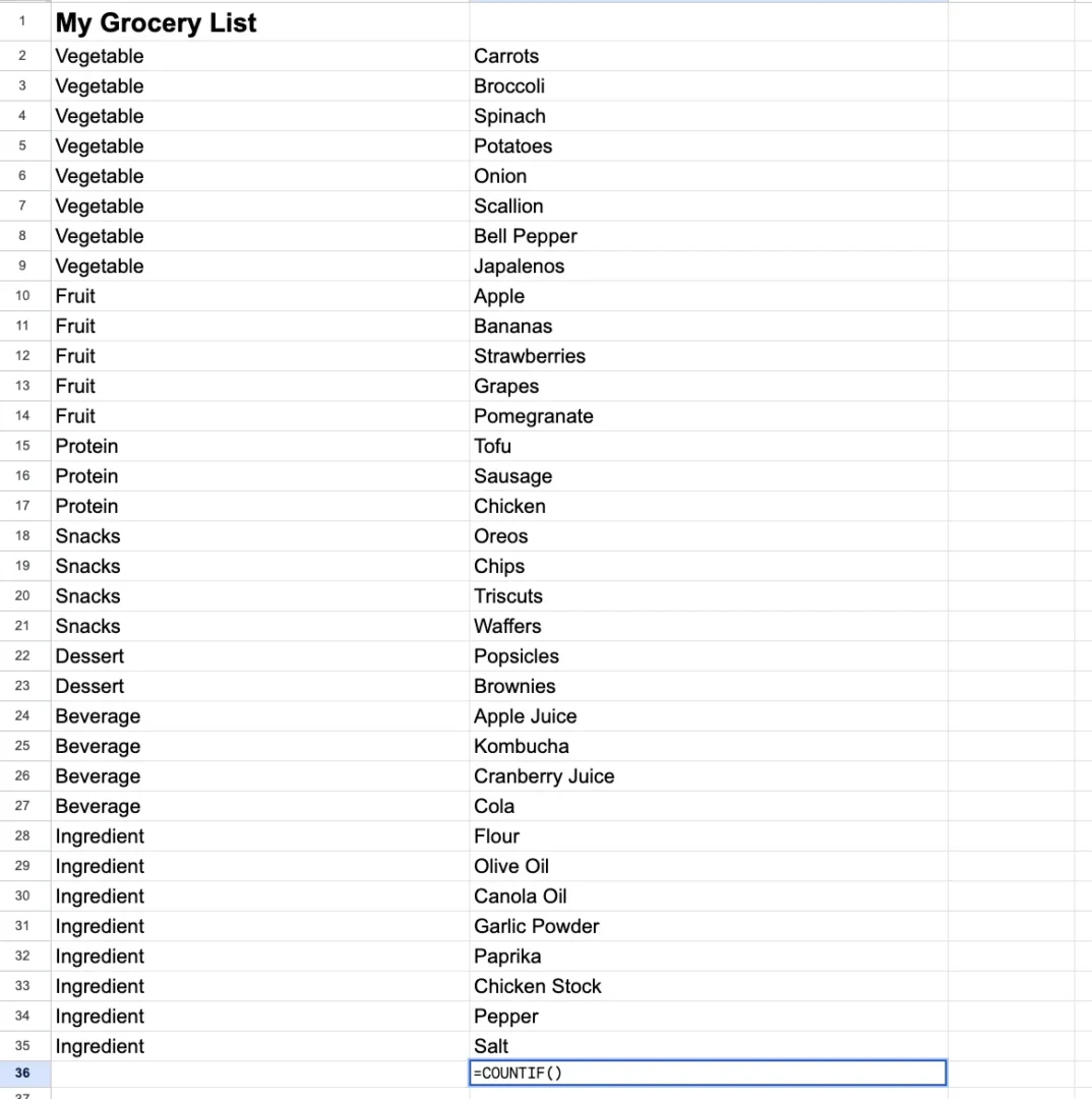
1. =COUNTIF()

Get started by the use of entering the following into the mobile where you want to position the answer:

=COUNTIF()

For this situation, we’ll use a grocery tick list that I’ve written. The opposite items I need to acquire are looked after by the use of type, like fruit and veggies.

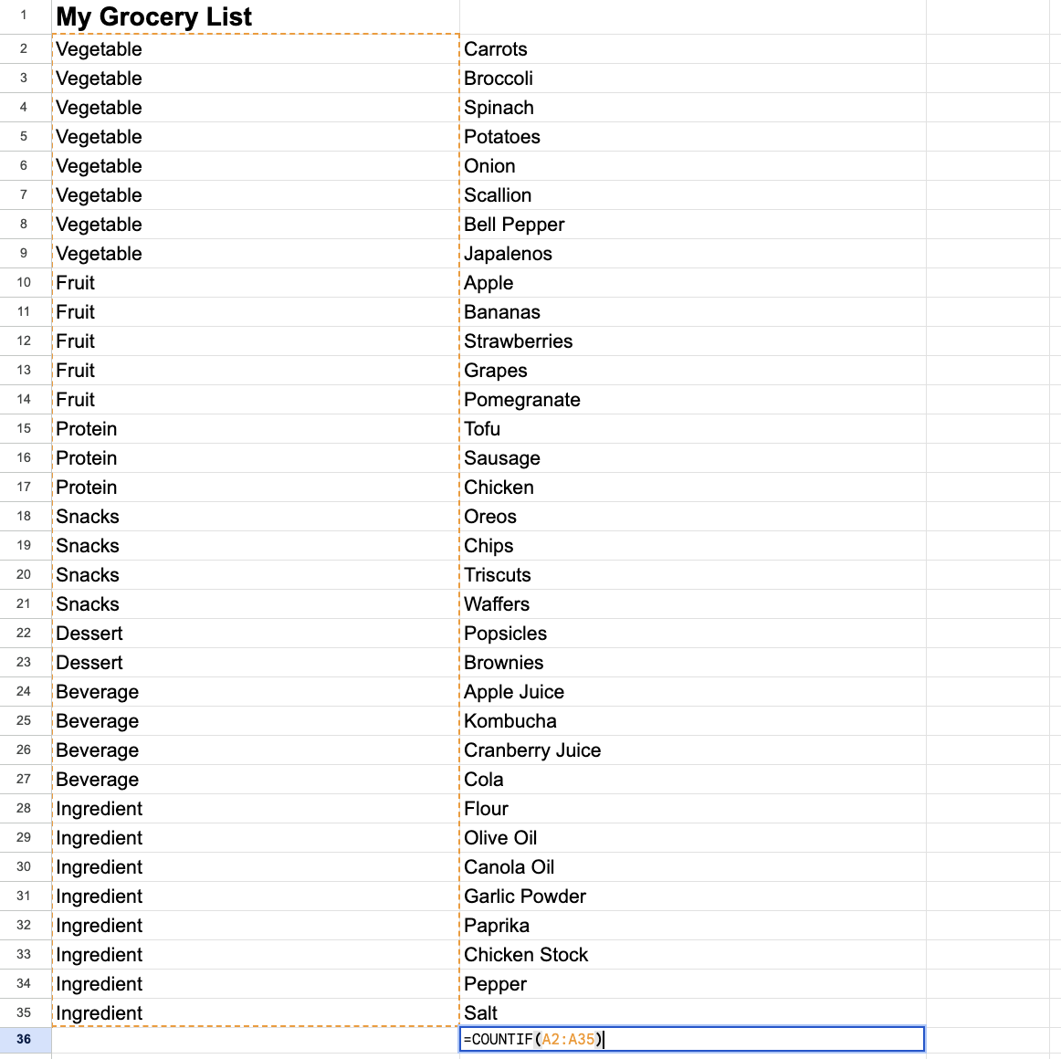
2. Define plenty of cells.

For the COUNTIF function to artwork, you should enter two arguments between the parentheses — the range of cells you’re looking at and the requirements you want to match.

Place your cursor all the way through the parentheses and each manually enter the range of cells (e.g., D1:D20) or use your mouse to highlight the range of cells in your spreadsheet.

Assuming your ZIP code values are in column D from row 1 to row 20, the function should now seem to be this:

=COUNTIF(A2:A35)

3. Add a comma.

Next, type a comma after the range, like this:

=COUNTIF(A2:A35,)

4. Define your search requirements.

You now need to enter the criteria or price that you want to rely after the comma, surrounded by the use of quotation marks.

In our example, let’s say you’re looking to appear what choice of vegetables are for your tick list. In this instance, the criteria you’re counting is Vegetable, and your function should now seem to be this:

=COUNTIF(A2:A35, “Vegetable“)

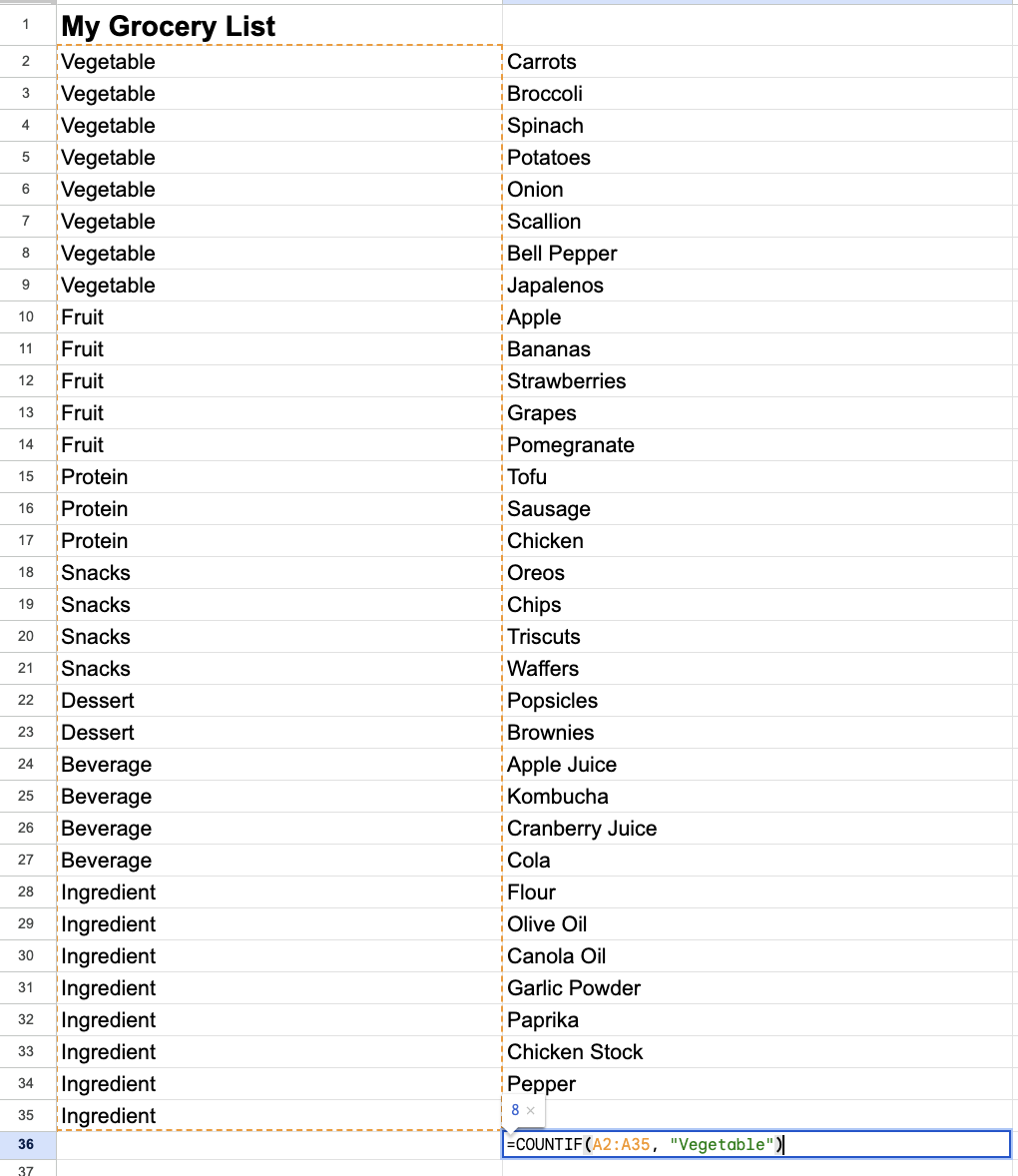
Apply that your requirements is generally a amount (“10”), text (“Los Angeles”), or another mobile (C3). Alternatively, in case you reference another mobile, you don’t surround it with quotation marks. Requirements aren’t case-sensitive, so it’s just right to enter “Crimson,” “pink,” or “RED” and get the equivalent results.

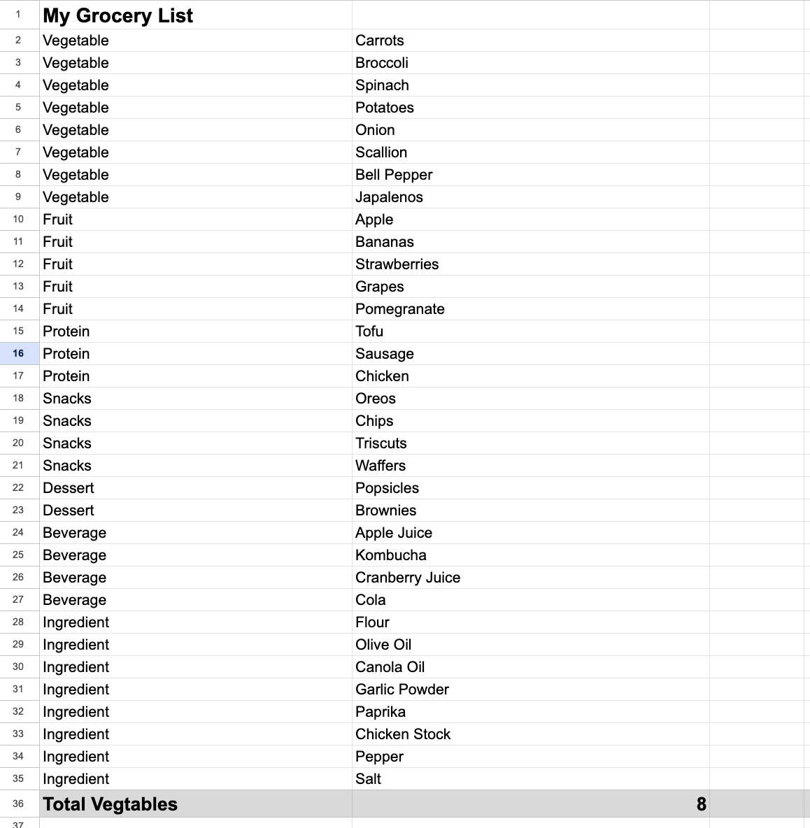
5. Flip at the function.

Press Enter, and the function activates, returning the choice of cells that suit your argument.

Tips for Using the COUNTIF Function

Many purchasers, myself built-in, have found out that you simply’ll have the ability to use the COUNTIF function in lots of more than a few tactics besides counting explicit values. Listed below are 3 tips I love to counsel for extending the use of the COUNTIF function.

Use wildcard characters for partial fits.

You don’t should reference a decided on price or requirements. Will have to you only know part of the price you want to rely, you’ll have the ability to use the * wildcard character to match any price in that part of the price.

For instance, let’s say you’ve were given an inventory of addresses. If you want to are compatible all ZIP codes that get began with the numbers 46 (related to 46032, 46033, and 46450), you want to enter 46 followed by the use of the * wildcard, like this:

=COUNTIF(D1:D20,“46*“)

You’ll use the wildcard character at each the beginning or the top of the price string. For instance, to rely all cells that end with the letters “polis,” enter the following:

=COUNTIF(D1:D20,“*polis“)

This will rely cells that include the cities of Indianapolis and Minneapolis.

Depend values which can also be greater than or less than a number.

Will have to you’re working with numbers, you could need to rely cells with values greater than or less than a given price. You do this by the use of using the mathematical greater than (>) and not more than (<) signs.

To rely all cells that have a price greater than a given amount, related to ten, enter this:

=COUNTIF(D1:D20,“>10“)

To rely cells which can also be greater than or an identical to a number, enter this:

=COUNTIF(D!:D20“>=10“)

To rely all cells that have a price less than a given amount, enter this:

=COUNTIF(D1:D20“<10“)

To rely cells that have a price less than or an identical to a given amount, enter this:

=COUNTIF(D1:D20“<=10“)

You’ll even rely cells with a price no longer an identical to a decided on amount. For instance, to rely cells that aren’t an identical to the volume 10, enter this:

=COUNTIF(D1:D20“10“)

In a lot of these instances, understand that the criteria, in conjunction with the less than, greater than, and an identical signs, should be enclosed within quotation marks.

Depend one price OR another.

The COUNTIF function can also be used to rely a few requirements—that is, cells that include one price or another.

For instance, likelihood is that you’ll need to rely customers who’re residing in each Los Angeles or San Diego. You do this by the use of using two COUNTIF functions with a + between them, like this:

=COUNTIF(D1:D20,“Los Angeles“)+COUNTIF(D1:D20,“San Diego“)

So that you can upload a lot more values, enter another + and COUNTIF function.

If you want to get a lot more out of Excel, check out our article on how one can use Excel like a professional. You’ll to search out 29 powerful tips, guidelines, and shortcuts that can make Excel much more straight forward to use.

Getting Started

Will have to you’re looking to rely the choice of items that are compatible explicit requirements, the COUNTIF function is learn to move. That you just should merely sort on that column and manually rely the entries, on the other hand using COUNTIF is an entire lot more straightforward.

Now, check it out and save yourself some time.

WordPress SEO

[ continue ]

WordPress Maintenance Plans | WordPress Hosting

read more