For lots of marketers, looking for to prepare and analyze spreadsheets in Microsoft Excel can in reality really feel like walking correct right into a brick wall time and again will have to you’e unfamiliar with Excel components. You’re manually replicating columns and scribbling down long-form math on a scrap of paper, all while thinking about in your self, “There has to be a better manner to try this.”

Truth be told, there is also — you merely don’t are aware of it however.

Excel can be tricky that manner. On the one hand, it’s an exceptionally tricky tool for reporting and analyzing promoting and advertising data. It would even assist you to visualize data with charts and pivot tables. On the other, without the right kind training, it’s easy to in reality really feel adore it’s running against you. For starters, there are more than a dozen vital formulation Excel can robotically run for you so that you at the moment are no longer combing through lots of cells with a calculator on your desk.

What are excel components?

Excel components assist you to determine relationships between values throughout the cells of your spreadsheet, perform mathematical calculations the usage of those values, and return the following value throughout the cellular of your variety. Method you’ll robotically perform include sum, subtraction, percentage, division, reasonable, and even dates/events.

We’re going to move over all of the ones, and a variety of additional, in this blog submit.

Learn how to Insert Method in Excel

You must marvel what the “Method” tab on the height navigation toolbar in Excel manner. In more moderen diversifications of Excel, this horizontal menu — confirmed beneath — means that you can to seek out and insert Excel components into specific cells of your spreadsheet. 

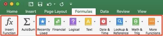
The additional you use moderately numerous components in Excel, the better it is going to be to remember them and perform them manually. Nonetheless, the suite of icons above is a to hand catalog of components you’ll browse and refer once more to as you hone your spreadsheet skills.

Excel components also are known as “functions.” To insert one into your spreadsheet, highlight a cellular during which you wish to have to run a components, then click on at the far-left icon, “Insert Function,” to browse commonplace components and what they do. That browsing window will seem to be this:

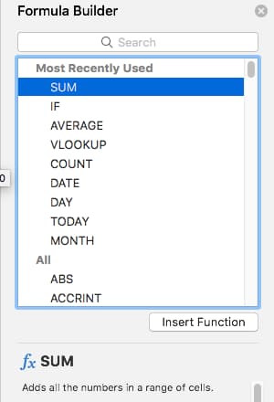Want a additional taken care of browsing revel in? Use any of the icons now we have now highlighted (all the way through the long pink rectangle throughout the first screenshot above) to go looking out components related to moderately a couple of common subjects — very similar to finance, commonplace sense, and additional. Once you’ve gotten found out the components that matches your needs, click on on “Insert Function,” as confirmed throughout the window above.

Now, let’s do a deeper dive into some of the necessary most crucial Excel components and the best way to perform each one in same old scenarios.

To help you use Excel additional effectively (and save a ton of time), now we have now compiled a listing of an important components, keyboard shortcuts, and other small guidelines and functions you’ll have to know.

NOTE: The following components practice to the latest style of Excel. If you’re the usage of a somewhat older style of Excel, the site of each serve as mentioned beneath might be somewhat different.

1. SUM  

All Excel components get started with the equals sign, =, followed thru a decided on text tag denoting the components you wish to have Excel to perform. 

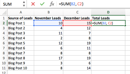
The SUM components in Excel is one of the most straightforward components you’ll enter correct right into a spreadsheet, allowing you to find the sum (or total) of two or additional values. To perform the SUM components, enter the values you wish to have in an effort to upload together the usage of the format, =SUM(value 1, value 2, and lots of others).

The values you enter into the SUM components can each be actual numbers or an identical to the volume in a decided on cellular of your spreadsheet. 

• To hunt out the SUM of 30 and 80, for instance, type the following components correct right into a cellular of your spreadsheet: =SUM(30, 80). Press “Enter,” and the cellular will produce the entire of each and every numbers: 110. 
• To hunt out the SUM of the values in cells B2 and B11, for instance, type the following components correct right into a cellular of your spreadsheet: =SUM(B2, B11). Press “Enter,” and the cellular will produce the entire of the numbers in this day and age filled in cells B2 and B11. If there aren’t any numbers in each cellular, the components will return 0. 

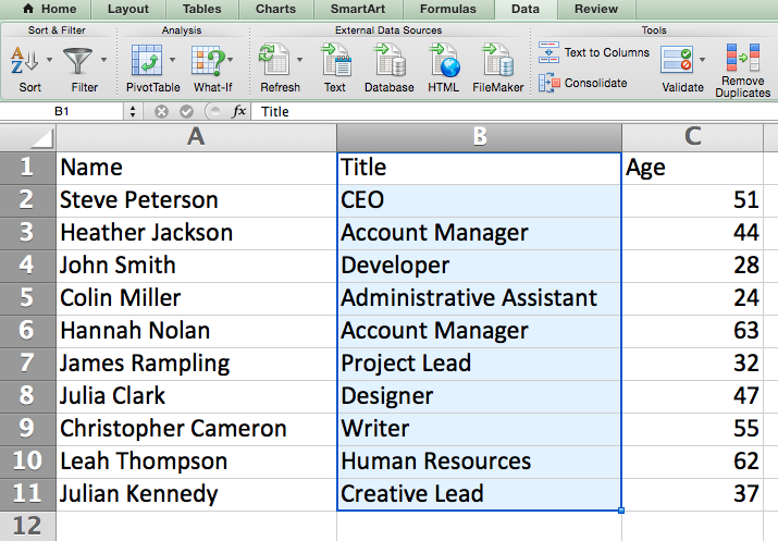
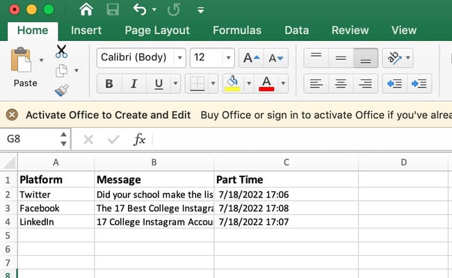
Consider you’ll moreover to seek out the entire value of a report of numbers in Excel. To hunt out the SUM of the values in cells B2 through B11, type the following components correct right into a cellular of your spreadsheet: =SUM(B2:B11). Understand the colon between each and every cells, rather than a comma. See how this might most likely look in an Excel spreadsheet for a content material subject material marketer, beneath:

2. IF

The IF components in Excel is denoted =IF(logical_test, value_if_true, value_if_false). This permits you to enter a text value into the cellular “if” something else on your spreadsheet is correct or false. As an example, =IF(D2=”Gryffindor”,”10&High;,”0&High;) would award 10 problems to cellular D2 if that cellular contained the word “Gryffindor.”

There are times after we want to know the way many times a price turns out in our spreadsheets. Alternatively there are also those events after we want to to seek out the cells that contain those values, and input specific data next to it.

We’re going to go back to Sprung’s example for this one. If we want to award 10 problems to everyone who belongs throughout the Gryffindor house, as a substitute of manually typing in 10’s next to each Gryffindor pupil’s determine, we’re going to make use of the IF-THEN components to say: If the scholar is in Gryffindor, then he or she must get ten problems.

• The components: IF(logical_test, value_if_true, value_if_false)
  • Logical_Test: The logical take a look at is the “IF” part of the commentary. In this case, the common-sense is D2=”Gryffindor.” Ensure that your Logical_Test value is in quotation marks.
  • Value_if_True: If the associated fee is correct — that is, if the scholar lives in Gryffindor — this value is the person who we want to be displayed. In this case, we might find it irresistible to be the volume 10, to indicate that the scholar was once as soon as awarded the 10 problems. Understand: Most effective use quotation marks if you wish to have the result to be text as a substitute of a host.
  • Value_if_False: If the associated fee is pretend — and the scholar does no longer live in Gryffindor — we would love the cellular to show “0,” for 0 problems.
• Elements in beneath example: =IF(D2=”Gryffindor”,”10&High;,”0&High;)

3. Proportion

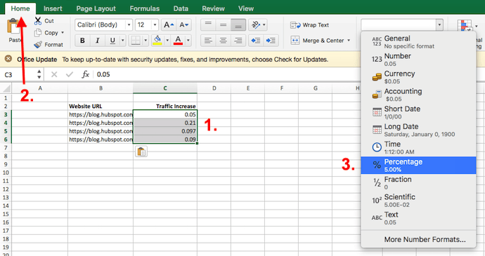
To perform the share components in Excel, enter the cells you might be finding a percentage for throughout the format, =A1/B1. To turn into the following decimal value to a percentage, highlight the cellular, click on at the Area tab, and make a choice “Proportion” from the numbers dropdown.

There isn’t an Excel “components” for percentages in line with se, alternatively Excel makes it easy to turn into the cost of any cellular correct right into a percentage so that you at the moment are no longer stuck calculating and reentering the numbers yourself.

The fundamental environment to turn into a cellular’s value correct right into a percentage is under Excel’s Area tab. Select this tab, highlight the cellular(s) you would really like to transform to a percentage, and click on on into the dropdown menu next to Conditional Formatting (this menu button would most likely say “Not unusual” to start with). Then, make a choice “Proportion” from the report of possible choices that appears. This will now and again convert the cost of each cellular you’ve gotten highlighted correct right into a percentage. See this selection beneath.

Consider if you’re the usage of other components, such for the reason that division components (denoted =A1/B1), to return new values, your values would most likely show up as decimals thru default. Simply highlight your cells faster than or after you perform this components, and set the ones cells’ format to “Proportion” from the Area tab — as confirmed above.

4. Subtraction

To perform the subtraction components in Excel, enter the cells you might be subtracting throughout the format, =SUM(A1, -B1). This will now and again subtract a cellular the usage of the SUM components thru together with a hostile sign faster than the cellular you might be subtracting. As an example, if A1 was once as soon as 10 and B1 was once as soon as 6, =SUM(A1, -B1) would perform 10 + -6, returning a price of 4.

Like percentages, subtracting does no longer have its private components in Excel each, alternatively that doesn’t indicate it can’t be completed. You’ll be capable to subtract any values (or those values inside cells) two other ways.

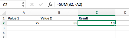
• Using the =SUM components. To subtract a few values from one each different, enter the cells you would really like to subtract throughout the format =SUM(A1, -B1), with a hostile sign (denoted with a hyphen) faster than the cellular whose value you might be subtracting. Press enter to return the variation between each and every cells built-in throughout the parentheses. See how this seems throughout the screenshot above.
• Using the format, =A1-B1. To subtract a few values from one each different, simply type an equals sign followed thru your first value or cellular, a hyphen, and the associated fee or cellular you might be subtracting. Press Enter to return the variation between each and every values.

5. Multiplication

To perform the multiplication components in Excel, enter the cells you might be multiplying throughout the format, =A1*B1. This components uses an asterisk to multiply cellular A1 thru cellular B1. As an example, if A1 was once as soon as 10 and B1 was once as soon as 6, =A1*B1 would return a price of 60.

You must suppose multiplying values in Excel has its private components or uses the “x” persona to suggest multiplication between a few values. In reality, it is so simple as an asterisk — *.

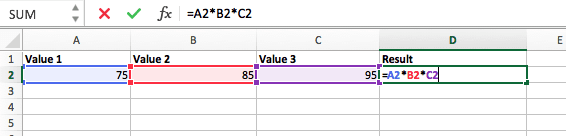
To multiply two or additional values in an Excel spreadsheet, highlight an empty cellular. Then, enter the values or cells you wish to have to multiply together throughout the format, =A1*B1*C1 … and lots of others. The asterisk will effectively multiply each value built-in throughout the components.

Press Enter to return your desired product. See how this seems throughout the screenshot above.

6. Division

To perform the dept components in Excel, enter the cells you might be dividing throughout the format, =A1/B1. This components uses a forward slash, “/,” to divide cellular A1 thru cellular B1. As an example, if A1 was once as soon as 5 and B1 was once as soon as 10, =A1/B1 would return a decimal value of 0.5.

Division in Excel is one of the most straightforward functions you’ll perform. To do so, highlight an empty cellular, enter an equals sign, “=,” and apply it up with the two (or additional) values you would really like to divide with a forward slash, “/,” in between. The outcome must be throughout the following format: =B2/A2, as confirmed throughout the screenshot beneath.

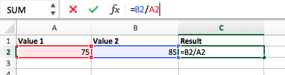
Hit Enter, and your desired quotient must appear throughout the cellular you initially highlighted.

7. DATE

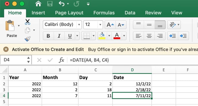
The Excel DATE components is denoted =DATE(year, month, day). This components will return a date that corresponds to the values entered throughout the parentheses — even values referred from other cells. As an example, if A1 was once as soon as 2018, B1 was once as soon as 7, and C1 was once as soon as 11, =DATE(A1,B1,C1) would return 7/11/2018.

Rising dates throughout the cells of an Excel spreadsheet is normally a fickle procedure every so often. Thankfully, there’s a to hand components to make formatting your dates easy. There are two tactics to use this components:

• Create dates from a series of cellular values. To do this, highlight an empty cellular, enter “=DATE,” and in parentheses, enter the cells whose values create your desired date — starting with the year, then the month amount, then the day. The total format must seem to be this: =DATE(year, month, day). See how this seems throughout the screenshot beneath.
• Automatically set in recent years’s date. To do this, highlight an empty cellular and enter the following string of text: =DATE(YEAR(TODAY()), MONTH(TODAY()), DAY(TODAY())). Pressing enter will return the existing date you might be running on your Excel spreadsheet.

In each usage of Excel’s date components, your returned date must be inside the kind of “mm/dd/yy” — till your Excel program is formatted otherwise.

8. Array

An array components in Excel surrounds a simple components in brace characters the usage of the format, {=(Get began Value 1:End Value 1)*(Get began Value 2:End Value 2)}. By means of pressing ctrl+shift+heart, this may occasionally more and more calculate and return value from a few ranges, rather than just explicit individual cells added to or multiplied thru one each different.

Calculating the sum, product, or quotient of explicit individual cells is discreet — merely use the =SUM components and enter the cells, values, or range of cells you wish to have to do so arithmetic on. Alternatively what about a few ranges? How do you in finding the combined value of a giant staff of cells?

Numerical arrays are a useful method to perform a few components at the equivalent time in a single cellular so that you’ll see one final sum, difference, product, or quotient. If you’re looking to go looking out total product sales profits from quite a few purchased units, for instance, the array components in Excel may be very right for you. This is how you could possibly do it:

1. To begin out the usage of the array components, type “=SUM,” and in parentheses, enter the first of two (or 3, or 4) ranges of cells you would really like to multiply together. Here’s what your enlargement would most likely seem to be: =SUM(C2:C5
2. Next, add an asterisk after the ultimate cellular of the main range you built-in on your components. This stands for multiplication. Following this asterisk, enter your 2nd range of cells. You’ll be multiplying this 2nd range of cells thru the main. Your enlargement in this components must now seem to be this: =SUM(C2:C5*D2:D5)
3. Ready to press Enter? Not so fast … On account of this components is so tricky, Excel reserves a definite keyboard command for arrays. Once you’ve gotten closed the parentheses on your array components, press Ctrl+Shift+Enter. This will now and again recognize your components as an array, wrapping your components in brace characters and successfully returning your made of each and every ranges combined.

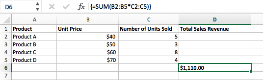
In profits calculations, this may occasionally decrease down on your time and effort significantly. See the overall components throughout the screenshot above.

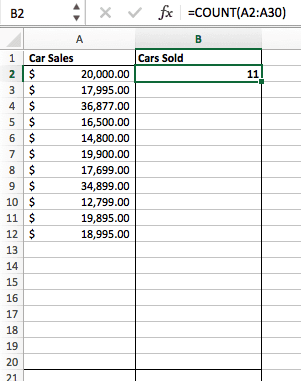
9. COUNT

The COUNT components in Excel is denoted =COUNT(Get began Cell:End Cell). This components will return a price that is equal to the choice of entries found out inside your desired range of cells. As an example, if there are 8 cells with entered values between A1 and A10, =COUNT(A1:A10) will return a price of 8.

The COUNT components in Excel is particularly useful for huge spreadsheets, in which you wish to have to see what choice of cells contain actual entries. Don’t be fooled: This components won’t do any math on the values of the cells themselves. This components is just to be told the best way many cells in a determined on range are thinking about something.

Using the components in bold above, you’ll merely run a rely of vigorous cells on your spreadsheet. The outcome will look quite something like this:

10. AVERAGE

To perform the everyday components in Excel, enter the values, cells, or range of cells of which you might be calculating the everyday throughout the format, =AVERAGE(number1, number2, and lots of others.) or =AVERAGE(Get began Value:End Value). This will now and again calculate the everyday of the entire values or range of cells built-in throughout the parentheses.

Finding the everyday of a range of cells in Excel assists in keeping you from having to go looking out explicit individual sums and then performing a separate division equation on your total. Using =AVERAGE as your initial text get right of entry to, you’ll let Excel do the entire provide the effects you wish to have.

For reference, the everyday of a host of numbers is equal to the sum of those numbers, divided during the choice of items in that staff.

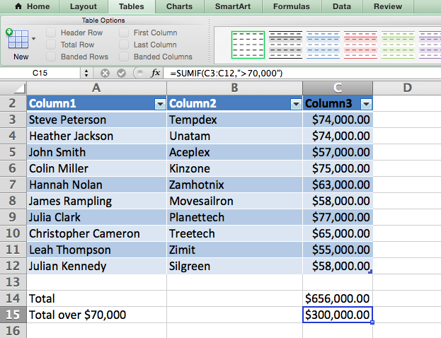
11. SUMIF

The SUMIF components in Excel is denoted =SUMIF(range, requirements, [sum range]). This will now and again return the sum of the values inside a desired range of cells that all meet one criterion. As an example, =SUMIF(C3:C12,”>70,000&High;) would return the sum of values between cells C3 and C12 from most straightforward the cells which may well be greater than 70,000.

Let’s imagine you wish to have to come to a decision the convenience you generated from a listing of leads who’re associated with specific area codes, or calculate the sum of positive staff’ salaries — alternatively only if they fall above a decided on amount. Doing that manually sounds quite time-consuming, to say the least.

With the SUMIF function, it does no longer wish to be — you’ll merely add up the sum of cells that meet positive requirements, like throughout the salary example above.

• The components: =SUMIF(range, requirements, [sum_range])
  
  • Range: The variability that is being tested the usage of your requirements.
  • Requirements: The standards that come to a decision which cells in Criteria_range1 can be added together
  • [Sum_range]: An optional range of cells you’re going to add up along side the main Range entered. This field is also pushed aside.

Throughout the example beneath, we had to calculate the sum of the salaries which were greater than $70,000. The SUMIF function added up the greenback amounts that exceeded that amount throughout the cells C3 through C12, with the components =SUMIF(C3:C12,”>70,000&High;).

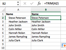
12. TRIM

The TRIM components in Excel is denoted =TRIM(text). This components will remove any spaces entered faster than and after the text entered throughout the cellular. As an example, if A2 comprises the determine ” Steve Peterson” with unwanted spaces faster than the main determine, =TRIM(A2) would return “Steve Peterson” and no longer the usage of a spaces in a brand spanking new cellular.

Electronic message and record sharing are wonderful apparatus in in recent years’s place of business. That is, until regarded as considered one of your colleagues sends you a worksheet with some in reality funky spacing. Not most straightforward can those rogue spaces make it tough to search for data, alternatively moreover they affect the results whilst you try to add up columns of numbers.

Somewhat than painstakingly eliminating and together with spaces as sought after, you’ll clean up any peculiar spacing the usage of the TRIM function, which is used to remove additional spaces from data (aside from for for single spaces between words).

• The components: =TRIM(text).
  • Text: The text or cellular from which you wish to have to remove spaces.

This is an example of the best way we used the TRIM function to remove additional spaces faster than a listing of names. To do so, we entered =TRIM(“A2”) into the Elements Bar, and replicated this for each determine beneath it in a brand spanking new column next to the column with unwanted spaces.

Underneath are any other Excel components you should to seek out useful as your data regulate needs expand.

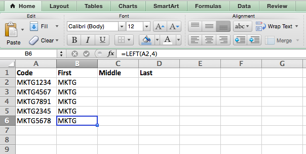
13. LEFT, MID, and RIGHT

Let’s imagine you should have a line of text inside a cellular that you wish to have to damage down into a few different segments. Somewhat than manually retyping each piece of the code into its respective column, shoppers can leverage a series of string functions to deconstruct the gathering as sought after: LEFT, MID, or RIGHT.

LEFT

• Goal: Used to extract the main X numbers or characters in a cellular.
• The components: =LEFT(text, number_of_characters)
  
  • Text: The string that you just need to extract from.
  • Number_of_characters: The choice of characters that you just need to extract starting from the left-most persona.

Throughout the example beneath, we entered =LEFT(A2,4) into cellular B2, and copied it into B3:B6. That allowed us to extract the main 4 characters of the code.

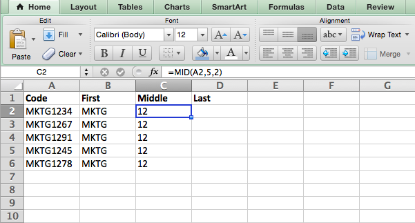
MID

• Goal: Used to extract characters or numbers throughout the middle in line with position.
• The components: =MID(text, start_position, number_of_characters)
  
  • Text: The string that you just need to extract from.
  • Start_position: The positioning throughout the string that you wish to have to begin out extracting from. As an example, the main position throughout the string is 1.
  • Number_of_characters: The choice of characters that you just need to extract.

In this example, we entered =MID(A2,5,2) into cellular B2, and copied it into B3:B6. That allowed us to extract the two numbers starting throughout the fifth position of the code.

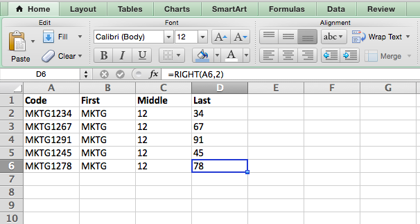
RIGHT

• Goal: Used to extract the ultimate X numbers or characters in a cellular.
• The components: =RIGHT(text, number_of_characters)
  
  • Text: The string that you just need to extract from.
  • Number_of_characters: The choice of characters that you wish to have to extract starting from the right-most persona.

For the sake of this example, we entered =RIGHT(A2,2) into cellular B2, and copied it into B3:B6. That allowed us to extract the ultimate two numbers of the code.

14. VLOOKUP

This one is an oldie, alternatively a goodie — and it’s more or less additional in depth than some of the necessary other components now we have now listed correct right here. Alternatively it’s in particular helpful for those events when you have two devices of information on two different spreadsheets, and want to combine them correct right into a single spreadsheet.

My colleague, Rachel Sprung — whose “The right way to Use Excel” tutorial is a must-read for somebody who needs to be informed — uses a listing of names, email addresses, and corporations for instance. If when you’ve got a listing of people’s names next to their email addresses in one spreadsheet, and a listing of those same people’s email addresses next to their company names throughout the other, alternatively you wish to have the names, email addresses, and company names of those people to seem in one place — that’s the position VLOOKUP is to be had in.

Understand: When the usage of this components, you will have to ensure a minimum of one column turns out identically in each and every spreadsheets. Scour your data devices to make sure the column of information you might be the usage of to combine your wisdom is precisely the equivalent, in conjunction with no additional spaces.

• The components: VLOOKUP(seek for value, table array, column amount, [range lookup])
  • Glance up Value: The an identical value you should have in each and every spreadsheets. Make a choice the main value on your first spreadsheet. In Sprung’s example that follows, this means the main email care for on the report, or cellular 2 (C2).
  • Table Array: The number of columns on Sheet 2 you’re going to pull your data from, in conjunction with the column of information similar to your seek for value (in our example, email addresses) in Sheet 1 along with the column of information you might be looking for to reproduction to Sheet 1. In our example, this is “Sheet2!A:B.” “A” manner Column A in Sheet 2, which is the column in Sheet 2 where the guidelines similar to our seek for value (email) in Sheet 1 is listed. The “B” manner Column B, which contains the guidelines this is most straightforward available in Sheet 2 that you wish to have to translate to Sheet 1.
  • Column Amount: The table array tells Excel where (which column) the new data you wish to have to duplicate to Sheet 1 is located. In our example, this would be the “Space” column, the second one in our table array, making it column amount 2.
  • Range Glance up: Use FALSE to you should definitely pull in most straightforward exact value suits.
• The components with variables from Sprung’s example beneath: =VLOOKUP(C2,Sheet2!A:B,2,FALSE)

In this example, Sheet 1 and Sheet 2 contain lists describing different information about the equivalent people, and the everyday thread between the two is their email addresses. Let’s imagine we want to combine each and every datasets so that the entire house wisdom from Sheet 2 translates over to Sheet 1. This is how that may art work:

15. RANDOMIZE

There’s a nice article that likens Excel’s RANDOMIZE components to shuffling a deck of enjoying playing cards. The entire deck is a column, and each card — 52 in a deck — is a row. “To shuffle the deck,” writes Steve McDonnell, “you’ll compute a brand spanking new column of information, populate each cellular throughout the column with a random amount, and type the workbook in line with the random amount field.”

In promoting and advertising, you should use this selection when you wish to have to assign a random amount to a listing of contacts — like will have to you wanted to experiment with a brand spanking new email advertising marketing campaign and had to use blind requirements to choose who would download it. By means of assigning numbers to said contacts, you should practice the guideline of thumb, “Any contact with a decide of 6 or above can be added to the new advertising marketing campaign.”

• The components: RAND()
  • Get began with a single column of contacts. Then, throughout the column adjacent to it, type “RAND()” — without the quotation marks — starting with the perfect contact’s row.
• • RANDBETWEEN means that you can dictate the number of numbers that you wish to have to be assigned. In terms of this example, I wanted to use one through 10.
  • bottom: The ground amount throughout the range.
  • height: The most productive conceivable amount throughout the range,For the example beneath: RANDBETWEEN(bottom,height)
  • Elements in beneath example: =RANDBETWEEN(1,10)

 

Helpful stuff, suitable? Now for the icing on the cake: Once you’ve gotten mastered the Excel components you wish to have, you’ll want to mirror it for various cells without rewriting the components. And unintentionally, there is also an Excel function for that, too. Check it out beneath.

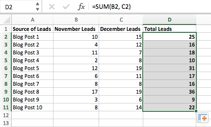
Once in a while, you should want to run the equivalent components all the way through an entire row or column of your spreadsheet. Let’s imagine, for instance, you have a listing of numbers in columns A and B of a spreadsheet and want to enter explicit individual totals of each row into column C.

Obviously, it is going to be too tedious to control the values of the components for each cellular so you might be finding the entire of each row’s respective numbers. Thankfully, Excel means that you can robotically whole the column; all you should do is enter the components throughout the first row. Check out the following steps: 

1. Kind your components into an empty cellular and press “Enter” to run the components.
2. Hover your cursor over the bottom-right corner of the cellular containing the components. You’ll see a small, bold “+” symbol appear.
3. While you’ll double-click this symbol to robotically fill all of the column in conjunction with your components, you’ll moreover click on on and drag your cursor down manually to fill only a specific duration of the column.Once you’ve gotten reached the ultimate cellular throughout the column you wish to have to enter your components, unlock your mouse to duplicate the components. Then, simply check each new value to make sure it corresponds to the right kind cells.

Excel Keyboard Shortcuts

1. In brief make a choice rows, columns, or all of the spreadsheet.

Most likely you might be crunched for time. I indicate, who isn’t? No time, no problem. You’ll be in a position to make a choice your entire spreadsheet in just one click on on. All you should do is just click on at the tab throughout the top-left corner of your sheet to concentrate on the entire thing swiftly.

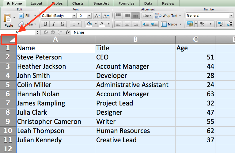
Merely want to choose the entire thing in a decided on column or row? This is merely as easy with the ones shortcuts:

For Mac:

• Select Column = Command + Shift + Down/Up
• Select Row = Command + Shift + Right kind/Left

For PC:

• Select Column = Keep an eye on + Shift + Down/Up
• Select Row = Keep an eye on + Shift + Right kind/Left

This shortcut is especially helpful when you’re running with higher data devices, alternatively most straightforward need to choose a decided on piece of it.

2. In brief open, close, or create a workbook.

Want to open, close, or create a workbook on the fly? The following keyboard shortcuts will help you whole any of the above actions in lower than a minute’s time.

For Mac:

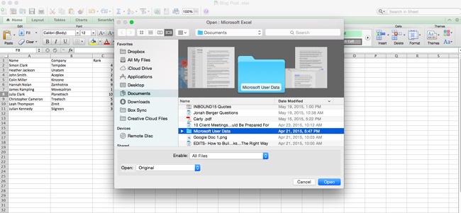
• Open = Command + O
• Close = Command + W
• Create New = Command + N

For PC:

• Open = Keep an eye on + O
• Close = Keep an eye on + F4
• Create New = Keep an eye on + N

3. Construction numbers into overseas cash.

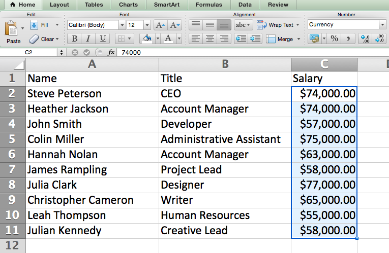
Have raw data that you wish to have to turn into overseas cash? Whether or not or no longer it’s salary figures, promoting and advertising budgets, or price ticket product sales for an match, the solution is unassuming. Merely highlight the cells you wish to have to reformat, and make a choice Keep an eye on + Shift + $.

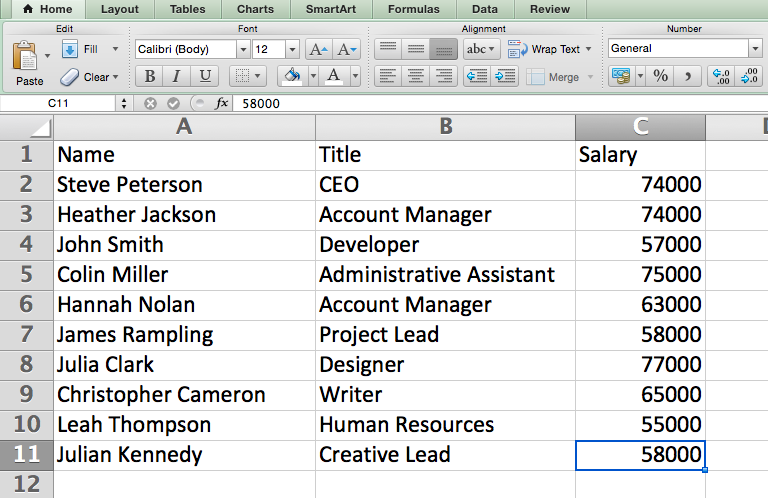
The numbers will robotically translate into greenback amounts — whole with greenback signs, commas, and decimal problems.

Understand: This shortcut moreover works with percentages. If you want to label a column of numerical values as “%” figures, alternate “$” with “%”.

4. Insert provide date and time correct right into a cellular.

Whether or not or no longer you might be logging social media posts, or keeping an eye on tasks you might be checking off your to-do report, you should want to add a date and time stamp to your worksheet. Get began thru settling at the cellular to which you wish to have in an effort to upload this knowledge.

Then, depending on what you wish to have to insert, do some of the necessary following:

• Insert provide date = Keep an eye on + ; (semi-colon)
• Insert provide time = Keep an eye on + Shift + ; (semi-colon)
• Insert provide date and time = Keep an eye on + ; (semi-colon), SPACE, and then Keep an eye on + Shift + ; (semi-colon).

Other Excel Pointers

1. Customize the color of your tabs.

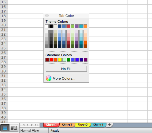
In case you have were given a ton of more than a few sheets in one workbook — which happens to the best folks — can help you determine where you wish to have to move thru color-coding the tabs. As an example, you should label ultimate month’s promoting and advertising critiques with pink, and this month’s with orange.

Simply suitable click on on a tab and make a choice “Tab Color.” A popup will appear that allows you to make a choice a color from an provide theme, or customize one to meet your needs.

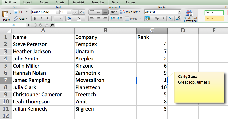
2. Add a commentary to a cellular.

When you wish to have to make an observation or add a commentary to a decided on cellular inside a worksheet, simply right-click the cellular you wish to have to the touch upon, then click on on Insert Commentary. Kind your commentary into the text box, and click on on outdoor the commentary box to reserve it.

Cells that contain comments display a small, pink triangle throughout the corner. To view the commentary, hover over it.

3. Copy and replica formatting.

Whilst you’ve ever spent some time formatting a sheet to your liking, you most likely agree that it isn’t exactly necessarily probably the most stress-free process. In fact, it’s stunning tedious.

Because of this, it’s more than likely that you don’t want to duplicate the process next time — nor do you should. Because of Excel’s Construction Painter, you’ll merely reproduction the formatting from one area of a worksheet to each different.

Select what you wish to have to duplicate, then make a choice the Construction Painter risk — the paintbrush icon — from the dashboard. The pointer will then display a paintbrush, prompting you to choose the cellular, text, or entire worksheet to which you wish to have to make use of that formatting, as confirmed beneath:

4. Decide copy values.

In a whole lot of instances, copy values — like copy content material subject material when managing SEO — can be tricky if lengthy long gone uncorrected. In some cases, despite the fact that, you simply need to concentrate on it.

Without reference to the situation is also, it’s easy to flooring any provide copy values inside your worksheet in just a few speedy steps. To do so, click on on into the Conditional Formatting risk, and make a choice Highlight Cell Regulations > Copy Values

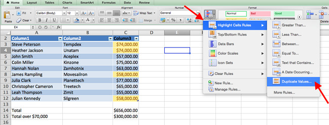
Using the popup, create the desired formatting rule to specify which type of copy content material subject material you wish to have to put across forward.

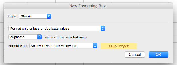
Throughout the example above, we have now been looking to identify any copy salaries all the way through the determined on range, and formatted the copy cells in yellow.

Excel Shortcuts Save You Time

In promoting and advertising, the use of Excel is gorgeous inevitable — alternatively with the ones guidelines, it does no longer wish to be so daunting. As they’re announcing, practice makes perfect. The additional you use the ones components, shortcuts, and guidelines, the additional they’re going to turn into 2nd nature.

Editor’s remember: This submit was once as soon as at first printed in January 2019 and has been up to the moment for comprehensiveness.

WordPress SEO

[ continue ]

WordPress Maintenance Plans | WordPress Hosting

read more